ACCES Tutorial#
Introduction#
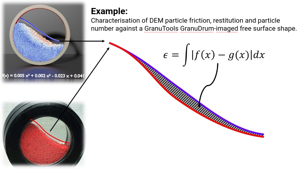
ACCES - or autonomous calibration and characterisation via evolutionary software - can calibrate virtually any simulation parameters against a user-defined cost function, quantifying and then minimising the “difference” between the simulated system and experimental reality – in essence, autonomously ‘learning’ the physical properties of the particles within the system, without the need for human input. This cost function is completely general, allowing ACCESS to calibrate simulations against measurements as simple as photographed occupancy plots, or complex system properties captured through e.g. Lagrangian particle tracking.
But what does this “difference between simulation and reality” look like? Damn awful:
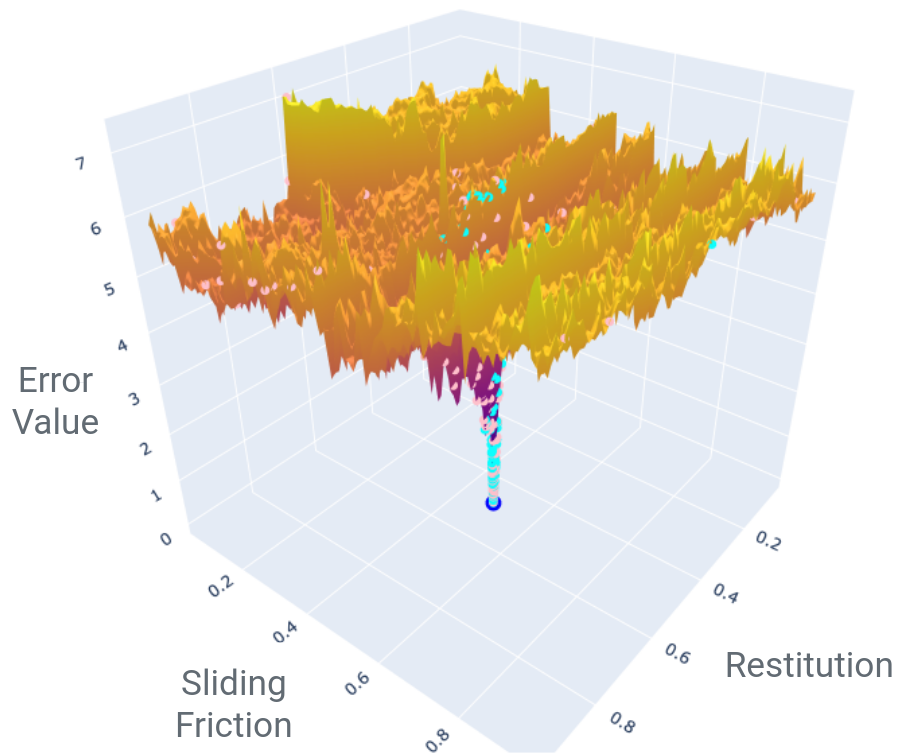
We ran the same DEM simulation of a vibrofluidised bed on a 100x100 grid of parameters (10,000 simulations indeed, thank you BlueBEAR @Birmingham), then compared central simulation’s occupancy profile with the other simulations.
Fundamentally, this is an optimisation problem: what parameters do I need such that my simulation reproduces an experimental measurement? But it is a horrible one, with the error function typically being noisy, non-smooth and having many false, local minima. In mathematical terms, it is non-convex and non-smooth - so gradient-based optimisers go out the window. Plus, a single simulation (a single point on the graph above) can take hours or days to run.
Enter CMA-ES [CMAES], a gradient-free global optimisation strategy that consistently ranks amongst the best optimisers for tough, global problems [OptBench] which forms the core of ACCES.
ACCES can take arbitrary Python scripts defining a simulation, automatically parallelise them to execute efficiently on multithreaded laptops or even distributed computing clusters and deterministically optimise the user-defined free parameters. It is fault-tolerant and can return to the latest optimisation state even after e.g. a system crash.
Hansen N, Müller SD, Koumoutsakos P. Reducing the time complexity of the derandomized evolution strategy with covariance matrix adaptation (CMA-ES). Evolutionary computation. 2003 Mar;11(1):1-8.
Rios LM, Sahinidis NV. Derivative-free optimization: a review of algorithms and comparison of software implementations. Journal of Global Optimization. 2013 Jul;56(3):1247-93.
Example ACCES Run#
Simulations are oftentimes huge beasts that are hard to set up and run correctly / efficiently; ask a modeller to re-write their simulation as a function (which is what virtually all optimisers expect) and you might not be friends anymore. ACCES takes a different approach: it accepts entire simulation scripts; so you can take even pre-existing simulations and just define the free parameters ACCES can vary at the top, e.g.:
# In file `simulation_script.py`

# ACCESS PARAMETERS START
import coexist

parameters = coexist.create_parameters(
    variables = ["CED", "CoR", "Epsilon", "Mu"],
    minimums = [-5, -5, -5, -5],
    maximums = [+5, +5, +5, +5],
    values = [0, 0, 0, 0],          # Optional, initial guess
)

access_id = 0                       # Optional, unique ID for each simulation
# ACCESS PARAMETERS END


# Extract the free parameters' values - ACCES will modify / optimise them.
x, y, z, t = parameters["value"]


# Define the error value in *any* way - run a simulation, analyse data, etc.
#
# For simplicity, here's an analytical 4D Himmelblau function with 8 global
# and 2 local minima - the initial guess is very close to the local one!
error = (x**2 + y - 11)**2 + (x + y**2 - 7)**2 + z * t
All you need to do is to create a variable called parameters (a simple
pandas.DataFrame) storing the free parameters’ names and bounds, and
optionally starting values and relative uncertainty. Then, by the end of
the simulation script, just define a variable named exactly error,
storing a number that will need to be minimised.
Importantly, the above simulation script can be run on its own - so
while prototyping your simulation, just run the script and see if a single
simulation works fine; if it does, then you can pass it to ACCES to
optimise the error:
# In file `access_learn.py`, same folder as `simulation_script.py`

import coexist

# Use ACCESS to learn a simulation's parameters
access = coexist.Access("simulation_script.py")
access.learn(
    num_solutions = 10,         # Number of solutions per epoch
    target_sigma = 0.1,         # Target std-dev (accuracy) of solution
    random_seed = 42,           # Reproducible / deterministic optimisation
)
You will get an output showing the parameter combinations being tried and corresponding error values:
================================================================================
Starting ACCES run at 13:05:47 on 02/03/2022 in directory `access_seed42`.
================================================================================
Epoch    0 | Population 10
--------------------------------------------------------------------------------
Scaled overall standard deviation: 1.0
             CED       CoR   Epsilon        Mu
estimate     0.0  0.000000  0.000000  0.000000
uncertainty  4.0  4.000050  4.000100  4.000150
scaled_std   1.0  1.000013  1.000025  1.000038

        CED       CoR   Epsilon        Mu       error
0  1.218868 -4.159988  3.001880  3.762400  331.093228
1 -3.095859 -4.967675  0.511374 -1.265018  252.732762
2 -0.067205 -3.412218  3.517680  3.111284  239.466423
3  0.264123  4.509021  1.870084 -3.437299  219.638764
4  1.475003 -3.835578  3.513889 -0.199711  243.967225
5 -0.739449 -2.723752  4.825957 -0.618141  170.752129
6 -1.713311 -1.408552  2.129290  1.461831  138.135979
7  1.650930  1.723306  2.333195 -1.625721   44.785098
8 -2.048971 -3.255132  2.463979  4.516059  114.660635
9 -0.455790 -3.360668 -3.298007  2.602469  206.454823
Total function evaluations: 10

================================================================================
Epoch    1 | Population 10
--------------------------------------------------------------------------------
Scaled overall standard deviation: 1.0346092474852793
                  CED       CoR   Epsilon        Mu
estimate    -0.154096 -0.641435  4.978669  0.731821
uncertainty  3.895601  3.679495  4.795107  4.013030
scaled_std   0.973900  0.919874  1.198777  1.003258

[...output truncated...]

================================================================================
Epoch   31 | Population 10
--------------------------------------------------------------------------------
Scaled overall standard deviation: 0.10326429766691796
                  CED       CoR   Epsilon        Mu
estimate     3.621098 -1.748473  4.999445 -4.992881
uncertainty  0.052355  0.078080  0.284105  0.180196
scaled_std   0.013089  0.019520  0.071026  0.045049

          CED       CoR   Epsilon        Mu      error
310  3.574473 -1.650134  4.999374 -4.901913 -23.996813
311  3.582026 -1.756384  4.863496 -4.973417 -24.071692
312  3.628789 -1.616891  4.859678 -4.992656 -23.386000
313  3.662351 -1.782704  4.982040 -4.998059 -24.478008
314  3.594971 -1.725715  4.999877 -4.898257 -24.269162
315  3.577725 -1.744971  4.998411 -4.956502 -24.629198
316  3.613914 -1.747412  4.983253 -4.996630 -24.690880
317  3.579212 -1.774811  4.852262 -4.972910 -24.055219
318  3.634952 -1.784927  4.999971 -4.999863 -24.783959
319  3.647169 -1.872419  4.999971 -4.978640 -24.685207
Total function evaluations: 320


Optimal solution found within `target_sigma`, i.e. 10.0%:
  sigma = 0.08390460663313563 < 0.1

================================================================================
The best result was found in 32 epochs:
              CED       CoR   Epsilon        Mu      error
  value  3.569249 -1.813354  4.995112 -4.994052 -24.920092
  sigma  0.042168  0.060116  0.203900  0.140874

These results were found for the job:
  access_seed42/results/parameters.284.pickle
================================================================================
Take a moment to appreciate what we’ve done here: out of 8 global and 2 local - false - minima, we have found an optimum 4-dimensional parameter combination with only 320 function evaluations. Compare that with a classical approach of regularly sampling on a 10x10x10x10 grid - we used 30 times fewer “simulations”, yet we found an optimum within 0.32% of the analytical solution!
Each ACCES run creates a folder “access_seed<random_seed>” saving the optimisation
state. You can access (pun intended) it using coexist.AccessData(),
even while the optimisation is still running for intermediate results:
>>> access_data = coexist.AccessData("access_seed42")
>>> access_data

AccessData
--------------------------------------------------------------------------------
paths             ╎ AccessPaths(...)
parameters        ╎             value  min  max     sigma
                  ╎ CED      3.569249 -5.0  5.0  0.052355
                  ╎ CoR     -1.813354 -5.0  5.0  0.078080
                  ╎ Epsilon  4.995112 -5.0  5.0  0.284105
                  ╎ Mu      -4.994052 -5.0  5.0  0.180196
parameters_scaled ╎             value   min   max     sigma
                  ╎ CED      0.892312 -1.25  1.25  0.013089
                  ╎ CoR     -0.453338 -1.25  1.25  0.019520
                  ╎ Epsilon  1.248778 -1.25  1.25  0.071026
                  ╎ Mu      -1.248513 -1.25  1.25  0.045049
scaling           ╎ [4. 4. 4. 4.]
population        ╎ 10
num_epochs        ╎ 32
target            ╎ 0.1
seed              ╎ 42
epochs            ╎ DataFrame(CED_mean, CoR_mean, Epsilon_mean, Mu_mean,
                  ╎           CED_std, CoR_std, Epsilon_std, Mu_std, overall_std)
epochs_scaled     ╎ DataFrame(CED_mean, CoR_mean, Epsilon_mean, Mu_mean,
                  ╎           CED_std, CoR_std, Epsilon_std, Mu_std, overall_std)
results           ╎ DataFrame(CED, CoR, Epsilon, Mu, error)
results_scaled    ╎ DataFrame(CED, CoR, Epsilon, Mu, error)
You can create a “convergence plot” showing the evolution of the ACCES run using
coexist.plots.access:
import coexist

# Use path to either the `access_seed<random_seed>` folder itself, or its
# parent directory
access_data = coexist.AccessData("access_seed42")

fig = coexist.plots.access(access_data)
fig.show()
Which will produce the following interactive Plotly figure:
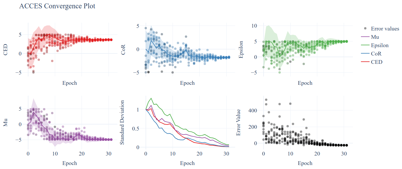
If you zoom into the error value, you’ll see that ACCES effectively found the optimum in less than 15 epochs; while this particular error function is smooth and a gradient-based optimiser may be quicker if the initial guess is close to a global optimum, this can never be assumed with physical simulations and noisy measurements (see the image at the top of the page).
You can visualise 2D slices through the parameter space explored, colour-coded by the error value of the closest parameter combination tried:
import coexist

# Use path to either the `access_seed<random_seed>` folder itself, or its
# parent directory
access_data = coexist.AccessData("access_seed42")

fig = coexist.plots.access2d(access_data)
fig.show()
Which will produce the following interactive Plotly figure:
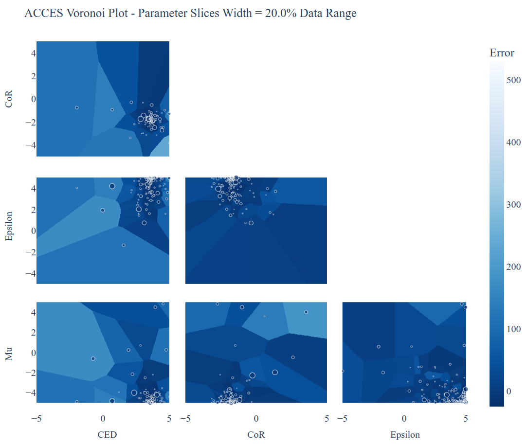
The dots are the parameter combinations tried; the cells’ colours represent the closest simulation’s error value (darker = smaller). The smaller the cell, the more simulations were run in that region - notice how ACCES spends minimum computational time on unimportant, high-error areas and more around the global optimum.
ACCES on Supercomputing Clusters#
ACCES can also run each simulation as separate, massively-parallel jobs on distributed
supercomputing clusters using the coexist.schedulers interface. For example, for
executing simulations as sbatch jobs on a SLURM-managed supercomputer (such as
the awesome BlueBEAR @Birmingham):
import coexist
from coexist.schedulers import SlurmScheduler


scheduler = SlurmScheduler(
    "10:0:0",           # Time allocated for a single simulation
    commands = '''
        # Commands you'd add in the sbatch script, after `#`
        set -e
        module purge; module load bluebear
        module load BEAR-Python-DataScience/2020a-foss-2020a-Python-3.8.2
    ''',
    qos = "bbdefault",
    account = "windowcr-rt-royalsociety",
    constraint = "cascadelake",     # Any other #SBATCH -- <CMD> = "VAL" pair
)

# Use ACCESS to learn the simulation parameters
access = coexist.Access("simulation_script.py", scheduler)
access.learn(num_solutions = 100, target_sigma = 0.1, random_seed = 12345)
Same script as before, except for the scheduler second argument to
coexist.Access. For full details - and extra possible settings - do check out
the “Manual” tab at the top of the page.